Prediction intervals

We can make two kinds of predictions from our model [Faraway (2002); Section 3.5]:

1. predictions about the “average” (“if we have some set of covariates, what is the average response given those covariates?”) – mean future predictions
2. predictions about specific situation (“we have some set of covariates, what is it’s prediction”) – predictions of future observations

In both cases the mean effect will be the same (so we can simply use the output from predict(model) but there are differences in how to calculate the uncertainty. In the latter case we need to include the additional variance from the error term in the model (usually denoted \(\epsilon\)). We call this second case a prediction interval.

Thinking about the normal response case (ignoring link functions etc for now), if we can write down the linear predictor of our model as \(\boldsymbol{X}\boldsymbol{\beta}\), we want \(\text{Var}(\boldsymbol{X}\boldsymbol{\beta})\) in case 1. above. For case 2. we have the prediction as \(\boldsymbol{X}\boldsymbol{\beta} + \epsilon\). \(\mathbf{E}(\epsilon) = 0\), so we ignore this for the mean effect, but we need to take \(\epsilon\) into account.

More generally, we want to take into account uncertainty from the various hyperparameters of the response distribution, like scale, shape etc.

It’s simplest to show this via posterior simulation, so that’s what is used here.

A general algorithm

We start with the posterior simulation template, so first let’s define some terms. \(\mathbf{X}_{p}\) is the matrix that maps parameters to their predictions on the linear predictor scale (the “\(L_p\) matrix” or “projection matrix”). \(\boldsymbol{\beta}\) is the vector of parameters from our fitted model and \(\mathbf{V}_{\hat{\boldsymbol{\beta}}}\) is its corresponding variance-covariance matrix. It’s also worth remembering that \(\boldsymbol{\beta}\) is approximately normally distributed (it’s exact for normal response), so we can use the multivariate normal distribution to generate \(\boldsymbol{\beta}\)s that are consistent with our model.

Regular posterior simulation is as follows:

1. For \(b=1,\ldots,B\):
2. Simulate from \(N(\hat{\boldsymbol{\beta}},\mathbf{V}_{\hat{\boldsymbol{\beta}}})\), to obtain \(\boldsymbol{\beta}_{b}\).
3. Calculate prediction \(Y^*_b=\mathbf{1}g^{-1}\left(\mathbf{X}_{p}\boldsymbol{\beta}_{b}\right)\)
4. Store \(Y_b^*\).
5. Calculate the empirical variance or percentiles of the \(Y_b^*\)s.

Now, to create a prediction interval, we adapt as follows:

1. For \(b=1,\ldots,B\):
2. Simulate from \(N(\hat{\boldsymbol{\beta}},\mathbf{V}_{\hat{\boldsymbol{\beta}}})\), to obtain \(\boldsymbol{\beta}_{b}\).
3. Calculate prediction \(Y^*_b=\mathbf{1}g^{-1}\left(\mathbf{X}_{p}\boldsymbol{\beta}_{b}\right)\)
4. Generate a random deviate from the response family with mean \(Y_b^*\) and other (hyper)parameters from the fitted model (scale, etc) to obtain \(Y^\dagger_b\).
5. Calculate the empirical variance or percentiles of the \(Y_b^\dagger\)s.

Our addition here is at point 3, generating random deviates from the response family. In the normal case, this just corresponds to generating using rnorm, mean generated from the simulated predictions and the variance using the estimated scale parameter (model$scale). For other distributions it may involve fewer scale parameters (e.g., Poisson) or more (e.g., Gamma).

Examples

The following code is adapted from this r-help mailing list post by Simon Wood with added comments for clarity.

Example 1 - normal response

For the first example, we’ll simulate some normally-distributed data using the gamSim function in mgcv, but only use one predictor, for simplicity.

library(mgcv)

Loading required package: nlme

This is mgcv 1.9-1. For overview type 'help("mgcv-package")'.

## simulate some data...
set.seed(8)
dat <- gamSim()

Gu & Wahba 4 term additive model

# just want one predictor here to make y just f2 + noise
dat$y <- dat$f2 + rnorm(400, 0, 1)

We can then fit an extremely boring model to this data:

## fit smooth model to x, y data...
b <- gam(y~s(x2,k=20), method="REML", data=dat)

Now to the central bit of the problem

## simulate replicate beta vectors from posterior...
n.rep <- 10000
br <- rmvn(n.rep, coef(b), vcov(b))

## turn these into replicate smooths
xp <- seq(0, 1, length.out=200)

# this is the "Lp matrix" which maps the coefficients to the predictors
# you can think of it like the design matrix but for the predictions
Xp <- predict(b, newdata=data.frame(x2=xp), type="lpmatrix")

# note that we should apply the link function here if we have one
# this is now a matrix with n.rep replicate smooths over length(xp) locations
fv <- Xp%*%t(br)

# now simulate from normal deviates with mean as in fv
# and estimated scale...
yr <- matrix(rnorm(length(fv), fv, b$scale), nrow(fv), ncol(fv))

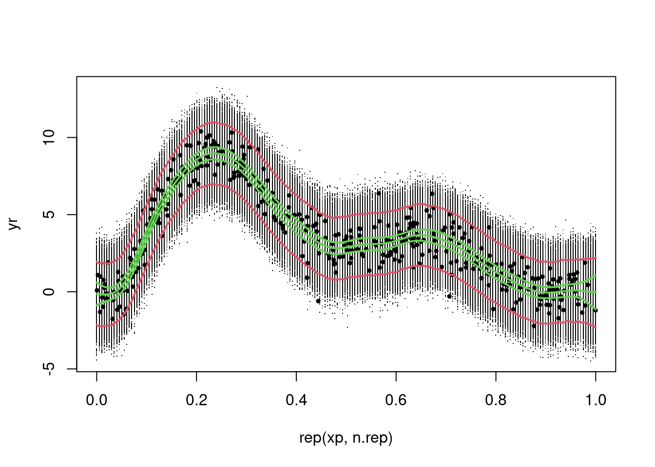
now make some plots

# plot the replicates in yr
plot(rep(xp, n.rep), yr, pch=".")
# and the data we used to fit the model
points(dat$x2, dat$y, pch=19, cex=.5)

# compute 95% prediction interval
# since yr is a matrix where each row is a data location along x2 and
# each column is a replicate we want the quantiles over the rows, summarizing
# the replicates each time
PI <- apply(yr, 1, quantile, prob=c(.025,0.975))
# the result has the 2.5% bound in the first row and the 97.5% bound
# in the second

# we can then plot those two bounds
lines(xp, PI[1,], col=2, lwd=2)
lines(xp, PI[2,], col=2, lwd=2)

# and optionally add the confidence interval for comparison...
pred <- predict(b, newdata=data.frame(x2=xp), se=TRUE)
lines(xp, pred$fit, col=3, lwd=2)
u.ci <- pred$fit + 2*pred$se.fit
l.ci <- pred$fit - 2*pred$se.fit
lines(xp, u.ci, col=3, lwd=2)
lines(xp, l.ci, col=3, lwd=2)

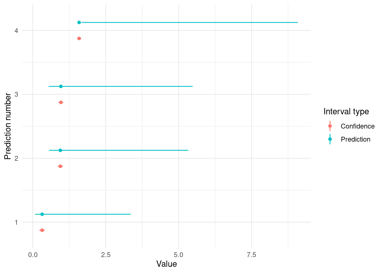
Example 2 - Tweedie response with multiple smooths

In this case we’re not going to plot smooths, but look at the prediction interval around a couple of predictions, to show that this method is very flexible.

library(mgcv)

# taken from ?mgcv::tw
set.seed(3)
n <- 400
## Simulate data...
dat <- gamSim(1, n=n, dist="poisson", scale=.2)

Gu & Wahba 4 term additive model

# using 2 terms to create the response
dat$y <- rTweedie(exp(dat$x2 + dat$x1), p=1.3, phi=.5)

We can then fit an extremely boring model to this data:

b2 <- gam(y~s(x2)+s(x1), family=tw(), data=dat)

## simulate replicate beta vectors from posterior...
n.rep <- 10000
br <- rmvn(n.rep, coef(b2), vcov(b2))

## turn these into replicate smooths
# here our prediction grid includes all variables, all of which are
# over 0,1
xp <- c(0.2, 0.8)
xp <- expand.grid(x2=xp, x1=xp)

# build the Lp matrix
Xp <- predict(b2, newdata=xp, type="lpmatrix")

# this is now a matrix with n.rep replicate smooths over length(xp)
# locations. Exponentiate to put on the response scale.
fv <- exp(Xp%*%t(br))

# now simulate from Tweedie deviates with mean exp(fv) (log link!),
# scale and power parameter from the model
yr <- matrix(rTweedie(fv, phi=b2$scale, p=b2$family$getTheta(TRUE)),
             nrow(fv), ncol(fv))

Now let’s calculate some intervals:

# compute 95% prediction interval
PI <- t(apply(yr, 1, quantile, prob=c(.025,0.975)))

# make regular predictions as usual
pred <- predict(b2, newdata=xp, se=TRUE)
tw_tab <- cbind.data.frame(prediction = pred$fit,
                lci = pred$fit - 1.96*pred$se.fit,
                uci = pred$fit + 1.96*pred$se.fit,
                PI)

We can put these in a table, here uci/lci are confidence intervals, 2.5%/97.5% indicate the prediction intervals, which are much wider.

knitr::kable(tw_tab)

prediction	lci	uci	2.5%	97.5%
0.3192804	0.2245227	0.4140381	0.0788077	3.350375
0.9439441	0.8548857	1.0330024	0.5585115	5.332643
0.9633439	0.8785245	1.0481634	0.5431233	5.479068
1.5880076	1.5171131	1.6589022	1.6711268	9.084479

Alternatively a plot shows this well:

library(ggplot2)

# a little manipulation to get this right
tw_tab_plot <- data.frame(prediction = rep(tw_tab$prediction, 2),
                          lci = c(tw_tab$lci, tw_tab[["2.5%"]]),
                          uci = c(tw_tab$uci, tw_tab[["97.5%"]]),
                          type = rep(c("Confidence", "Prediction"), each=4),
                          id = rep(1:4, 2))

ggplot(data=tw_tab_plot, aes(x=id, group=type, colour=type)) +
  geom_linerange(aes(y=prediction, ymin=lci, ymax=uci),
                 position=position_dodge2(width=0.5)) +
  geom_point(aes(y=prediction), position=position_dodge2(width=0.5)) +
  labs(y="Value", x="Prediction number", colour="Interval type") +
  coord_flip() +
  theme_minimal()

References

Faraway, J. J. (2002) Practical Regression and Anova using R.